VPRM timeseries

This tutorial will show you how to create timeseries of emission for the Vegetation Photosynthesis and Respiration Model (VPRM) within emiproc.

We will first prepare the input data, then run the model and finally visualize the results.

If you want to learn more how to use emiproc VPRM, you can check the documentation

import urllib.request

import pandas as pd
import matplotlib.pyplot as plt
from matplotlib.dates import MonthLocator, DateFormatter

from emiproc import  FILES_DIR
from emiproc.profiles.vprm import calculate_vprm_emissions


plt.style.use('default')

# Set up the working directory, change this if you want to check the files
# in a different location
work_dir = FILES_DIR / 'vprm'
work_dir.mkdir(exist_ok=True, parents=True)

Prepare input data

To run VPRM we need the following input data:

• Satellite data to calculate the vegetation indices

  • EVI: Enhanced Vegetation Index and

  • NDVI: Normalized Difference Vegetation Index

• Meteorological data (temperature and radiation)

• Vegetation parameters (constants for different vegetation types used in the model)

This tutorial will focus on the city of Zurich, which provide good open source data.

We will run vprm for the year 2024, with an hourly resolution. We won’t treat spatial resolution in this tutorial, so we are only interested in the temporal profiles.

Meteorological data

The city of zurich provides a good meteorological dataset, wo we can use this directly.

downlaod_link_meteo = "https://data.stadt-zuerich.ch/dataset/ugz_meteodaten_stundenmittelwerte/download/ugz_ogd_meteo_h1_2024.csv"
# Download the meteorological data
meteo_file = work_dir / 'meteo.csv'

if not meteo_file.is_file():
    urllib.request.urlretrieve(downlaod_link_meteo, meteo_file)

df_meteo = pd.read_csv(meteo_file, parse_dates=['Datum'])
df_meteo.head(10)

	Datum	Standort	Parameter	Intervall	Einheit	Wert	Status
0	2024-01-01 00:00:00+01:00	Zch_Heubeeribüel	Hr	h1	%Hr	89.95	bereinigt
1	2024-01-01 00:00:00+01:00	Zch_Heubeeribüel	T	h1	°C	3.23	bereinigt
2	2024-01-01 00:00:00+01:00	Zch_Heubeeribüel	p	h1	hPa	941.11	bereinigt
3	2024-01-01 00:00:00+01:00	Zch_Rosengartenstrasse	Hr	h1	%Hr	81.66	bereinigt
4	2024-01-01 00:00:00+01:00	Zch_Rosengartenstrasse	RainDur	h1	min	0.00	bereinigt
5	2024-01-01 00:00:00+01:00	Zch_Rosengartenstrasse	T	h1	°C	4.88	bereinigt
6	2024-01-01 00:00:00+01:00	Zch_Rosengartenstrasse	WD	h1	°	222.41	bereinigt
7	2024-01-01 00:00:00+01:00	Zch_Rosengartenstrasse	WVs	h1	m/s	0.80	bereinigt
8	2024-01-01 00:00:00+01:00	Zch_Rosengartenstrasse	WVv	h1	m/s	0.76	bereinigt
9	2024-01-01 00:00:00+01:00	Zch_Rosengartenstrasse	p	h1	hPa	961.99	bereinigt

For VPRM we need to extract the Temperature and radiation. So we will try to get the T and the StrGlo parameters from the data.

cols = {}
for var_in_data, var in {
    "T": "T",
    "StrGlo": "Rad",
}.items():

    mask_var = df_meteo["Parameter"] == var_in_data
    # Make the average over the different stations
    serie = df_meteo.loc[mask_var, ["Datum", "Wert"]].groupby("Datum").mean()['Wert']
    cols[var] = serie

df_meteo_cleaned = pd.concat(cols, axis=1)
# Put to utc
df_meteo_cleaned.index = df_meteo_cleaned.index.tz_convert('UTC').tz_localize(None)
df_meteo_cleaned

	T	Rad
Datum
2023-12-31 23:00:00	4.6075	0.02
2024-01-01 00:00:00	4.5350	0.01
2024-01-01 01:00:00	4.7275	0.01
2024-01-01 02:00:00	4.6750	0.02
2024-01-01 03:00:00	4.5000	0.02
...	...	...
2024-12-31 18:00:00	-0.6100	0.02
2024-12-31 19:00:00	-0.9900	0.02
2024-12-31 20:00:00	-1.0375	0.02
2024-12-31 21:00:00	-1.1550	0.02
2024-12-31 22:00:00	-0.9725	0.02

8784 rows × 2 columns

We can have a look at the data

fig, axes = plt.subplots(2, 1,sharex=True)
df_daily = df_meteo_cleaned.resample("d").mean()
axes[0].plot(df_daily.index, df_daily["T"], label="Temperature")
axes[0].set_ylabel("Temperature [°C]")
axes[0].legend()
axes[1].plot(df_daily.index, df_daily["Rad"], label="Global radiation")
axes[1].set_ylabel("Global radiation [W/m²]")
axes[1].legend()

<matplotlib.legend.Legend at 0x78189e48d8b0>

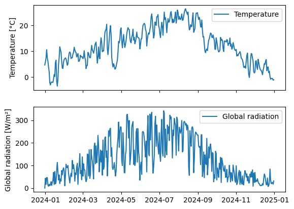
As expected, the temperature and radiation have daily fluctuations as well as seasonal ones.

It seems we can use that data for the next steps.

Satellite indicies

We will use the EVI and LSWI indices to calculate the vegetation parameters.

Usually you would need to download some satellite data and calculate the indices yourself. Then you will get the indices for different moment in the year.

This is a bit tedious, so here we will simply use some timeseries that are already generated. In case you want to do it yourself, you can follow this python tutorial

The satellite indices are not always given directly, if you need to calculate them, you can use the emiproc function calculate_vegetation_indices

df_sat = pd.read_csv(work_dir / "vegetation_indices.csv", index_col=0, header=[0, 1],
                 parse_dates=True)
df_sat

	Cropland		Deciduous		Evergreen		Grassland
	evi	lswi	evi	lswi	evi	lswi	evi	lswi
2021-01-24	NaN	NaN	NaN	NaN	0.318	0.686	NaN	NaN
2021-02-20	0.478	0.261	NaN	NaN	0.380	0.334	0.484	0.223
2021-02-23	0.444	0.265	NaN	NaN	0.292	0.380	0.499	0.256
2021-02-25	0.469	0.238	0.279	0.034	0.302	0.389	0.555	0.274
2021-03-02	0.494	0.240	0.235	-0.046	0.318	0.413	0.567	0.253
...	...	...	...	...	...	...	...	...
2025-04-15	NaN	NaN	NaN	NaN	NaN	NaN	0.971	0.450
2025-04-23	0.568	0.428	0.585	0.378	0.389	0.448	0.823	0.464
2025-04-27	NaN	NaN	0.407	0.396	NaN	NaN	0.887	0.424
2025-04-28	0.670	0.438	0.584	0.403	0.353	0.382	0.752	0.460
2025-04-30	0.652	0.443	0.746	0.425	0.440	0.411	0.827	0.461

302 rows × 8 columns

This table contains the evi and ndvi indices for different vegetation types at different days in time (where a satellite pass was available).

df_sat.loc["2024"].plot(linestyle="", marker='o', figsize=(10, 5))

<Axes: >

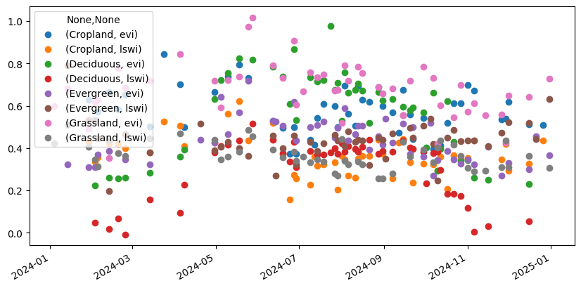
We need to interpolate the data to get estimates for the whole year. Since it is very stochastic, we use a robust method to interpolate the data.

# monthly median
df_sat_monthly_mean = df_sat.resample("MS").median()
# Add 15 days to be at the middle of the month
df_sat_monthly_mean.index = df_sat_monthly_mean.index + pd.Timedelta(days=15)
# Resample to hourly data and interpolate for the missing values
df_sat_full = df_sat_monthly_mean.resample("h").interpolate(method="akima").reindex(
    df_meteo_cleaned.index
)

ax = df_sat_full.plot(figsize=(10, 5))
ax.legend(loc="upper right", bbox_to_anchor=(1.25, 1))

<matplotlib.legend.Legend at 0x78189e957080>

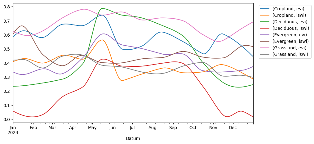
This is a very rough estimate, but most of the important features are captured.

We see lower values in the winter and higher values in the summer. Cropland has a huge drop in summer, which can happen when the crops are harvested.

Vegetation parameters

For the parameters, we will use the original parameters from the VPRM paper.

df_indices_mahadevan = pd.read_csv(work_dir / "vprm_parameters.csv", index_col="Site")
df_indices_mahadevan

	Tmin	Topt	Tmax	Tlow	PAR0	lambda	alpha	beta	std-PAR0	std-lambda	std-alpha	std-beta
Site
HARVARD	0	20	40	5.0	570	0.127	0.271	0.25	14	0.002	0.006	0.060
HOWLAND	0	20	40	2.0	629	0.123	0.244	-0.24	17	0.002	0.004	0.036
NOBS	0	20	40	1.0	262	0.234	0.244	0.14	5	0.004	0.002	0.015
NIWOT	0	20	40	1.0	446	0.128	0.250	0.17	13	0.003	0.003	0.018
METOLIUS	0	20	40	2.0	1206	0.097	0.295	-0.43	39	0.002	0.003	0.028
SOY_MEADS2	5	22	40	2.0	2051	0.064	0.209	0.20	137	0.002	0.005	0.058
CORN_MEAD	5	22	40	2.0	11250	0.075	0.173	0.82	1746	0.002	0.006	0.081
TONZI	2	20	40	0.0	3241	0.057	0.012	0.58	293	0.002	0.002	0.036
VAIRA	2	18	40	0.0	542	0.213	0.028	0.72	23	0.006	0.002	0.035
DONALDSON	0	20	40	1.0	790	0.114	0.153	1.56	18	0.002	0.004	0.076
LUCKY-HILLS	2	20	40	0.0	321	0.122	0.028	0.48	14	0.004	0.001	0.019
PEATLAND	0	20	40	3.0	558	0.051	0.081	0.24	23	0.002	0.002	0.019

Run VPRM

Now that we have all the input data, we can run VPRM.

This is simply done by calling the function calculate_vprm_emissions . If you look at the documentation, you can also see the equations used.

# Put all the timeseries together
df_vprm = df_sat_full.copy()
df_vprm[('T', 'global')] = df_meteo_cleaned['T']
df_vprm[('RAD', 'global')] = df_meteo_cleaned['Rad']
df_vprm

	Cropland		Deciduous		Evergreen		Grassland		T	RAD
	evi	lswi	evi	lswi	evi	lswi	evi	lswi	global	global
Datum
2023-12-31 23:00:00	0.585600	0.408814	0.233792	0.057975	0.335923	0.604519	0.623039	0.418926	4.6075	0.02
2024-01-01 00:00:00	0.585762	0.408886	0.233794	0.057870	0.335838	0.604807	0.622966	0.418943	4.5350	0.01
2024-01-01 01:00:00	0.585925	0.408958	0.233795	0.057766	0.335754	0.605095	0.622893	0.418960	4.7275	0.01
2024-01-01 02:00:00	0.586088	0.409029	0.233797	0.057661	0.335669	0.605382	0.622820	0.418977	4.6750	0.02
2024-01-01 03:00:00	0.586251	0.409101	0.233798	0.057557	0.335585	0.605669	0.622747	0.418994	4.5000	0.02
...	...	...	...	...	...	...	...	...	...	...
2024-12-31 18:00:00	0.445183	0.286038	0.245662	0.015723	0.374151	0.514763	0.691655	0.297948	-0.6100	0.02
2024-12-31 19:00:00	0.444992	0.285928	0.245715	0.015602	0.374239	0.514695	0.691764	0.297909	-0.9900	0.02
2024-12-31 20:00:00	0.444801	0.285817	0.245768	0.015482	0.374327	0.514627	0.691873	0.297869	-1.0375	0.02
2024-12-31 21:00:00	0.444610	0.285707	0.245822	0.015362	0.374415	0.514559	0.691982	0.297829	-1.1550	0.02
2024-12-31 22:00:00	0.444418	0.285597	0.245875	0.015241	0.374503	0.514490	0.692091	0.297790	-0.9725	0.02

8784 rows × 10 columns

# Choose which site to use for each category (rename the index)
# Of course this is not what you should do
# in a real application you should optimize the model to find the best parameters
# but since we are just doing a tutorial, we will use the default parameters
veg_mapping = {
        "NOBS": "Evergreen",
        "HARVARD": "Deciduous",
        "CORN_MEAD": "Cropland",
        "VAIRA": "Grassland",

    }
df_indices = df_indices_mahadevan.rename(
    index=veg_mapping
)
df_indices

	Tmin	Topt	Tmax	Tlow	PAR0	lambda	alpha	beta	std-PAR0	std-lambda	std-alpha	std-beta
Site
Deciduous	0	20	40	5.0	570	0.127	0.271	0.25	14	0.002	0.006	0.060
HOWLAND	0	20	40	2.0	629	0.123	0.244	-0.24	17	0.002	0.004	0.036
Evergreen	0	20	40	1.0	262	0.234	0.244	0.14	5	0.004	0.002	0.015
NIWOT	0	20	40	1.0	446	0.128	0.250	0.17	13	0.003	0.003	0.018
METOLIUS	0	20	40	2.0	1206	0.097	0.295	-0.43	39	0.002	0.003	0.028
SOY_MEADS2	5	22	40	2.0	2051	0.064	0.209	0.20	137	0.002	0.005	0.058
Cropland	5	22	40	2.0	11250	0.075	0.173	0.82	1746	0.002	0.006	0.081
TONZI	2	20	40	0.0	3241	0.057	0.012	0.58	293	0.002	0.002	0.036
Grassland	2	18	40	0.0	542	0.213	0.028	0.72	23	0.006	0.002	0.035
DONALDSON	0	20	40	1.0	790	0.114	0.153	1.56	18	0.002	0.004	0.076
LUCKY-HILLS	2	20	40	0.0	321	0.122	0.028	0.48	14	0.004	0.001	0.019
PEATLAND	0	20	40	3.0	558	0.051	0.081	0.24	23	0.002	0.002	0.019

df_emissions = calculate_vprm_emissions(
    df=df_vprm,
    df_vprm=df_indices,

)

Missing HOWLAND in the observation dataframe, skipping
Missing NIWOT in the observation dataframe, skipping
Missing METOLIUS in the observation dataframe, skipping
Missing SOY_MEADS2 in the observation dataframe, skipping
Missing TONZI in the observation dataframe, skipping
Missing DONALDSON in the observation dataframe, skipping
Missing LUCKY-HILLS in the observation dataframe, skipping
Missing PEATLAND in the observation dataframe, skipping

Plot VPRM results

Now we have another function that helps us to visualize the results.

Average daily cycle for each month

from emiproc.plots.vprm import plot_vprm_params_per_veg_type


plot_vprm_params_per_veg_type(df_emissions, df_indices, group_by='%m%H')

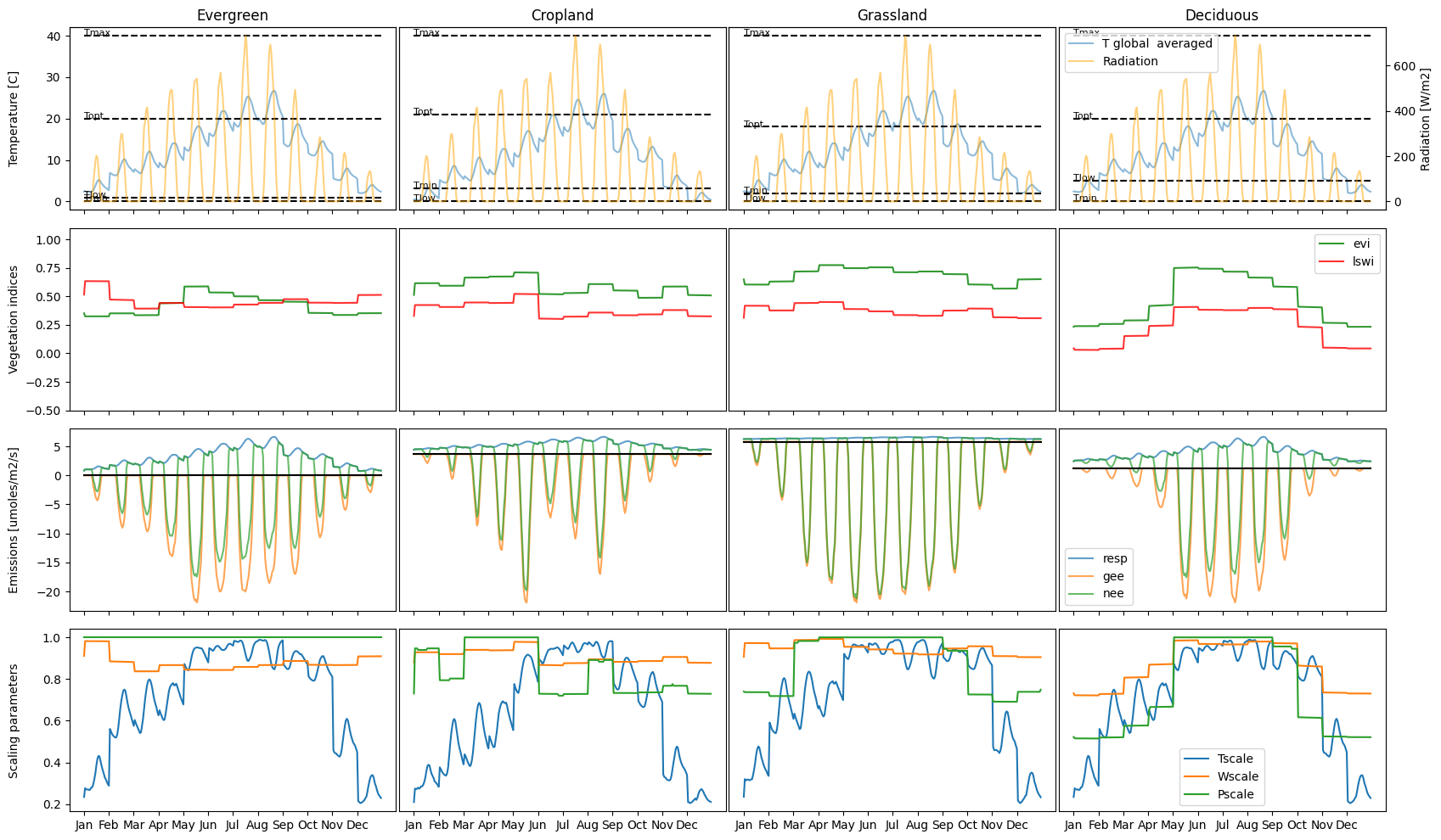
We see nice diurnal cycles, which are stronger in summer.

Different other parameters are shown to help us understand the results.

Daily means

plot_vprm_params_per_veg_type(df_emissions, df_indices, group_by='%m%d')

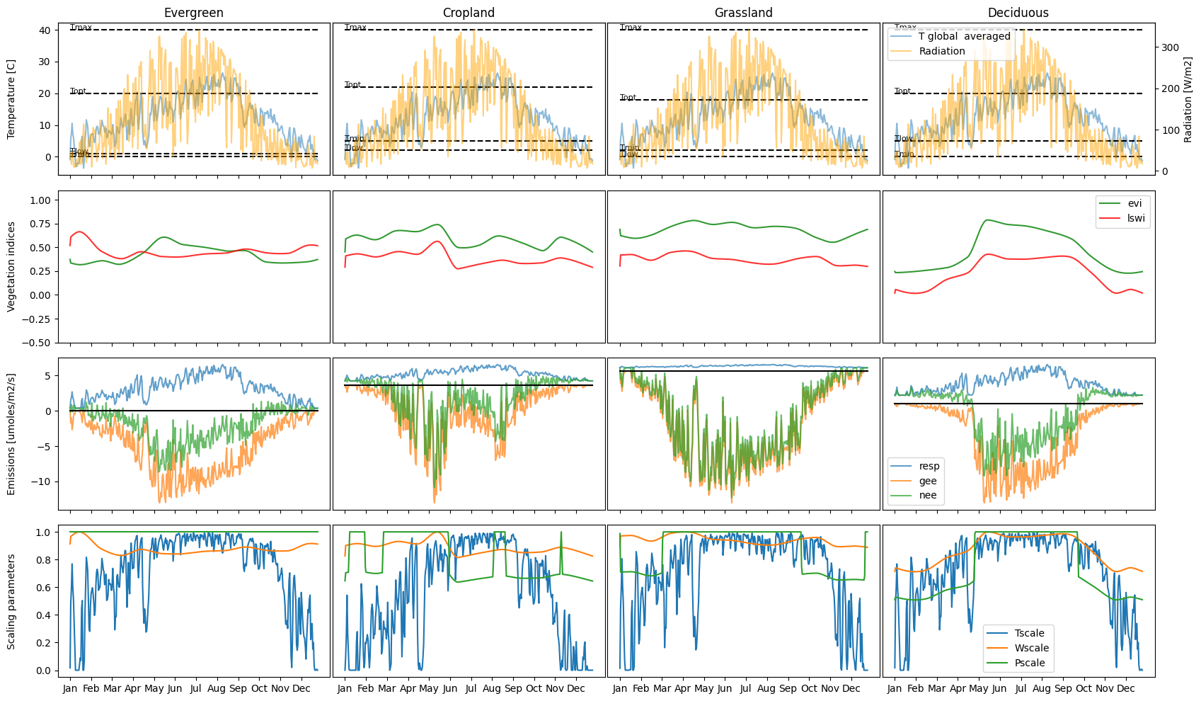
VPRM models

There exist different vprm models which change the equations slightly. Here we will look at some of them.

Urban vprm

The urban vprm is a modified version of the original vprm, which takes into account the urban heat island effect. For this a higher temperature is used as urban. It is nice in practice to have temperature sensors in the city to get a better estimate of the urban temperature.

In our data previously, we had different sites to use. Heubeeribüel is a bit outside of the city, so we will use that as global temperature. For the urban temperature we can use the Stampfenbachstrasse site, which is in the city center.

global_T = df_meteo.loc[(df_meteo['Standort'] == 'Zch_Heubeeribüel')  & (df_meteo['Parameter'] == 'T')][['Datum', 'Wert']].set_index('Datum')['Wert']
urban_T = df_meteo.loc[(df_meteo['Standort'] == 'Zch_Stampfenbachstrasse')  & (df_meteo['Parameter'] == 'T')][['Datum', 'Wert']].set_index('Datum')['Wert']


global_T.index = global_T.index.tz_convert('UTC').tz_localize(None)
urban_T.index = urban_T.index.tz_convert('UTC').tz_localize(None)

df_vprm_urban = df_vprm.copy()

df_vprm_urban[('T', 'global')] = global_T
df_vprm_urban[('T', 'urban')] = urban_T

fig, axes = plt.subplots(figsize=(10, 5), ncols=2)
for label in ['urban', 'global']:
    df_vprm_urban[('T', label)].plot(ax=axes[0], label=label, alpha=0.7)
    df_vprm_urban[('T', label)].groupby(df_vprm_urban.index.hour).mean().plot(ax=axes[1], label=label, alpha=0.7)
axes[0].legend()
axes[1].set_xlabel("Hour of the day")

Text(0.5, 0, 'Hour of the day')

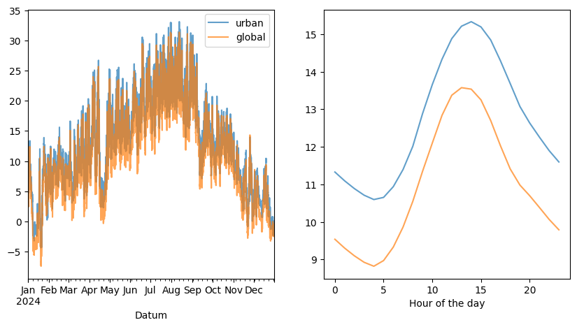
We can see that the global temperature is lower than the urban temperature.

Note that here we also have temperature difference due to altitude difference, but we will ignore that for now.

Impervious surface area (isa)

In cities, there are often large areas that are impervious (concrete, asphalt, buildings, etc.). This blocks the soil respiration and also affects the vegetation.

To account for this, we can use the impervious surface area (isa) model. if the isa fraction is 1, there is no soil respiration, if it is 0, there is full soil respiration (like in the normal model).

In a real case, you would split the vegetation by the isa fraction ( eg. street trees vs park trees would have different isa fractions )

For this tutorial we will simply assume that all vegetation has an isa fraction of 0.5.

df_indices['isa'] = 0.5
df_indices

	Tmin	Topt	Tmax	Tlow	PAR0	lambda	alpha	beta	std-PAR0	std-lambda	std-alpha	std-beta	resp_min	isa
Site
Deciduous	0	20	40	5.0	570	0.127	0.271	0.25	14	0.002	0.006	0.060	1.605	0.5
HOWLAND	0	20	40	2.0	629	0.123	0.244	-0.24	17	0.002	0.004	0.036	0.248	0.5
Evergreen	0	20	40	1.0	262	0.234	0.244	0.14	5	0.004	0.002	0.015	0.384	0.5
NIWOT	0	20	40	1.0	446	0.128	0.250	0.17	13	0.003	0.003	0.018	0.420	0.5
METOLIUS	0	20	40	2.0	1206	0.097	0.295	-0.43	39	0.002	0.003	0.028	0.160	0.5
SOY_MEADS2	5	22	40	2.0	2051	0.064	0.209	0.20	137	0.002	0.005	0.058	0.618	0.5
Cropland	5	22	40	2.0	11250	0.075	0.173	0.82	1746	0.002	0.006	0.081	1.166	0.5
TONZI	2	20	40	0.0	3241	0.057	0.012	0.58	293	0.002	0.002	0.036	0.580	0.5
Grassland	2	18	40	0.0	542	0.213	0.028	0.72	23	0.006	0.002	0.035	0.720	0.5
DONALDSON	0	20	40	1.0	790	0.114	0.153	1.56	18	0.002	0.004	0.076	1.713	0.5
LUCKY-HILLS	2	20	40	0.0	321	0.122	0.028	0.48	14	0.004	0.001	0.019	0.480	0.5
PEATLAND	0	20	40	3.0	558	0.051	0.081	0.24	23	0.002	0.002	0.019	0.483	0.5

EVI reference

Since the EVI measured in a urban context can be different from the real EVI, the urban model also include a reference EVI value, which is subtracted from the measured EVI.

for this example we will simply scale down the evi for reference.

for veg_type in veg_mapping.values():
    df_vprm_urban[(veg_type, 'evi_ref')] = df_vprm[(veg_type, 'evi')]
    df_vprm_urban[(veg_type, 'evi')] = df_vprm[(veg_type, 'evi')] * 0.8

from emiproc.profiles.vprm import VPRM_Model


df_emissions_urban = calculate_vprm_emissions(
    df=df_vprm_urban,
    df_vprm=df_indices,
    model=VPRM_Model.urban
)
df_emissions_urban.head()

Missing HOWLAND in the observation dataframe, skipping
Missing NIWOT in the observation dataframe, skipping
Missing METOLIUS in the observation dataframe, skipping
Missing SOY_MEADS2 in the observation dataframe, skipping
Missing TONZI in the observation dataframe, skipping
Missing DONALDSON in the observation dataframe, skipping
Missing LUCKY-HILLS in the observation dataframe, skipping
Missing PEATLAND in the observation dataframe, skipping

	Cropland		Deciduous		Evergreen		Grassland		T	RAD	...	Cropland	Grassland
	evi	lswi	evi	lswi	evi	lswi	evi	lswi	global	global	...	nee	resp_e_init	resp_h	resp_a	Tscale	Wscale	Pscale	resp	gee	nee
Datum
2023-12-31 23:00:00	0.468480	0.408814	0.187034	0.057975	0.268738	0.604519	0.498432	0.418926	3.23	0.02	...	1.448338	0.86644	0.21661	0.538745	0.407826	0.970681	0.306681	0.755355	-0.000510	0.754845
2024-01-01 00:00:00	0.468610	0.408886	0.187035	0.057870	0.268670	0.604807	0.498373	0.418943	3.16	0.01	...	1.443898	0.86560	0.21640	0.538245	0.404651	0.970693	0.306362	0.754645	-0.000253	0.754392
2024-01-01 01:00:00	0.468740	0.408958	0.187036	0.057766	0.268603	0.605095	0.498315	0.418960	3.57	0.01	...	1.456877	0.86812	0.21703	0.539835	0.414143	0.970705	0.306043	0.756865	-0.000259	0.756606
2024-01-01 02:00:00	0.468870	0.409029	0.187037	0.057661	0.268535	0.605382	0.498256	0.418977	3.37	0.02	...	1.453872	0.86756	0.21689	0.539509	0.412042	0.970716	0.305724	0.756399	-0.000514	0.755885
2024-01-01 03:00:00	0.469001	0.409101	0.187039	0.057557	0.268468	0.605669	0.498198	0.418994	3.06	0.02	...	1.433458	0.86364	0.21591	0.537094	0.397202	0.970728	0.305406	0.753004	-0.000495	0.752509

5 rows × 52 columns

Now we can compare the urban model with the normal model.

plot_vprm_params_per_veg_type(df_emissions, df_indices, group_by='%m%H')
plot_vprm_params_per_veg_type(df_emissions_urban, df_indices, group_by='%m%H', model=VPRM_Model.urban)

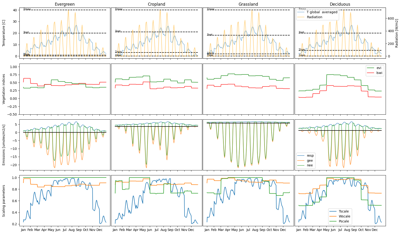
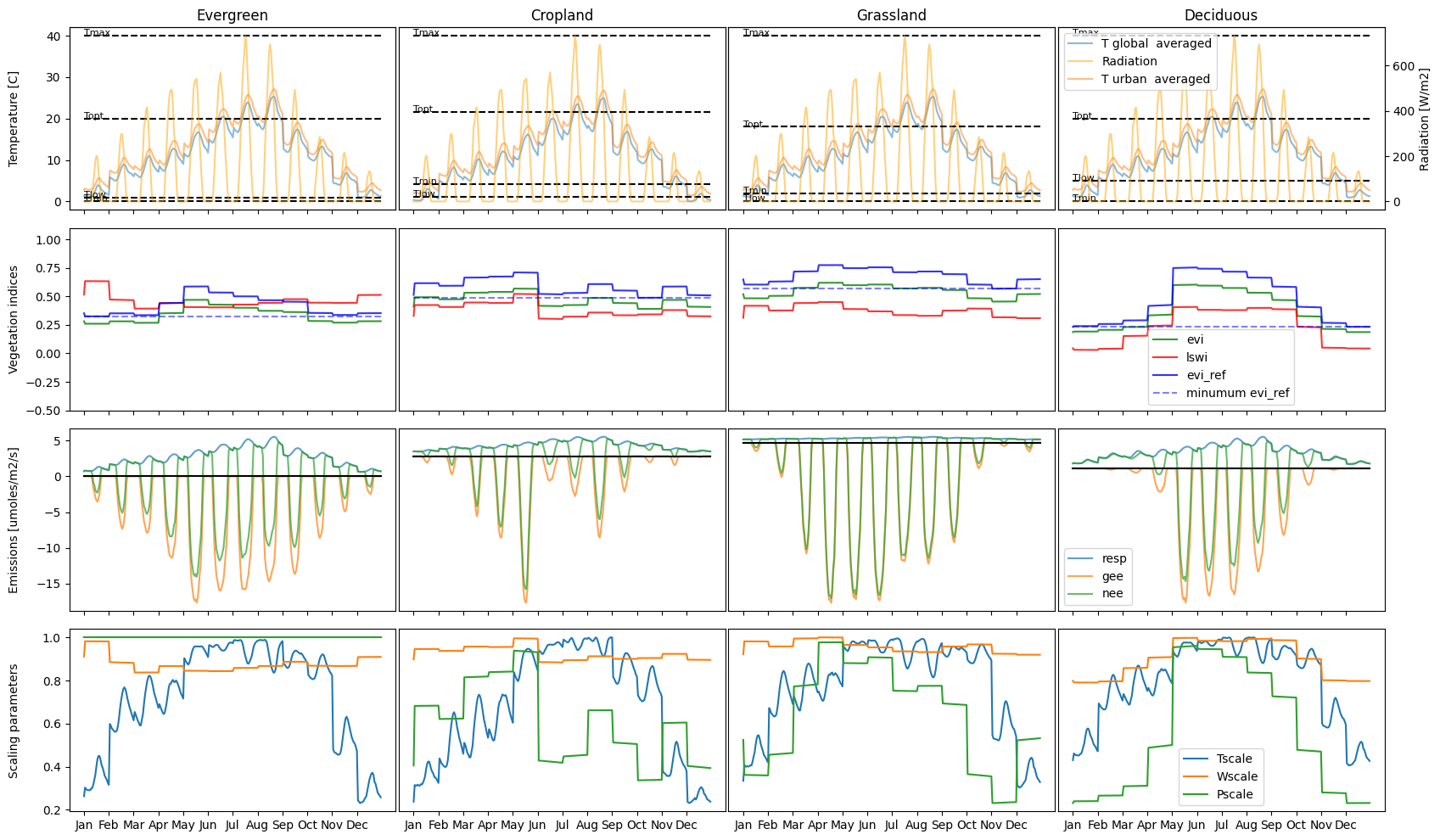
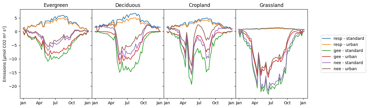
We can see that a first difference resides in the P scale, which is different for the urban model.

They claim to have a more realistic formulation which produces more realistic seasonal behaviour. It tranlates into lower total respiration and photosynthesis (plot below).

# Compare the total emissions over the year for both models
fig, axes = plt.subplots(
    figsize=(16, 4),
    ncols=len(veg_mapping) + 1,
    sharey=True,
    sharex=True,
    gridspec_kw={"wspace": 0},
)
legend_elements = []
for ax, veg_type in zip(axes[:-1], veg_mapping.values()):
    ax.set_title(f"{veg_type}")
    for var in ["resp", "gee", "nee"]:
        weekly_averages = {}
        for vprm_type, df_emis in {
            "standard": df_emissions,
            "urban": df_emissions_urban,
        }.items():
            weekly_avg = df_emis[(veg_type, var)].resample("W").mean()
            weekly_averages[vprm_type] = weekly_avg
        for label, serie in weekly_averages.items():
            line = ax.plot(serie.index, serie.values, label=f"{var} - {label}")
            if ax == axes[0]:
                legend_elements.append(line[0])

# Put the legennd in the last axis

axes[-1].legend(handles=legend_elements, loc="center")
axes[-1].axis("off")

# Ticks show only months
axes[0].xaxis.set_major_locator(MonthLocator(bymonth=range(1, 13, 3)))
axes[0].xaxis.set_major_formatter(DateFormatter("%b"))

axes[0].set_ylabel("Emissions [µmol CO2 m² s¹]")
plt.show()