Emission Profiles
Most of the inventories provide annual values for the emissions of a specific region. For simulations we need to know how they vary with time and elevation.
For that we downscale the annual values using profiles.
The total emission \(E\) is the sum of the emission for an emission source. It is given in \(kg/year/source\). Sources can be assigned profiles to describe how the emission varies with time and height.
We then can split the profiles in \(N\) intervals of time or height.
Scaling factors vs Ratios
There are two ways of describing the profiles:
Scaling factors
Ratios
Ratios signify the proportion of the total emission \(E\) that is emitted at a specific interval of time or height.
\(r_i\) the ratio at index \(i\) we have
Scaling factor give a value for which we can multiply the average emmission to get the emission at a specific time or height.
\(f_i\) is the scaling factor at index \(i\)
Based on these formulas, we can easily convert from one to the other.
Ratios sum up to one. Scaling factors have an average of one.
Emiproc stores internally ratios for the profiles, but uses and exports sometimes scaling factors.
scaling factors have the advantage that you can easily use them to combine profiles together.
Vertical Profiles
Vertical profiles in emiproc are handled by the class
VerticalProfile
Each inventory is assigned a set of profile, which can be attributed to a specific substance, category, gridcell or time .
Depending on how the data is gathered, different emission sources will have different profiles. In exemple a powerplant will emit at just one height.
When applying operations (regridding, groupping, …) on the inventories, the profiles might need to be changed as well.
Vertical data in emiproc is always the height over the ground.
Temporal Profiles
Fundamentally there are 2 ways of defining the time profile.
Deterministic
Periodic
Either you have an emission factor at a each time, creating a time serie for the emission.
Or you have periodic patterns that define patterns of behaviour (hour of day, day of week, mounth of year)
Creating profiles
To create the profiles, emiproc gives you some helper functions available in the API .
A notebook is also available : profiles.ipynb
Profiles in inventories
This chapter explains the format of the profiles in the inventories. The next chapter will explain how to assign the profiles to emissions.
In the inventory, the profiles will be stored as a
VerticalProfiles for vertical profiles.
This class is assigned to the v_profiles attribute of the inventory.
The temporal profiles are stored as a list of list of TemporalProfile.
They are assinged to the t_profiles_groups attribute of the inventory.
Each element of the main list is a list containing different types of temporal profiles object. We call this a group of temporal profiles.
# example of temporal profiles
t_profiles_groups = [
    # profile 0
    [
        WeeklyProfile(size=7, ratios=array([0.15, 0.15, 0.15, 0.15, 0.15, 0.12, 0.12])),
        DailyProfile(size=24, ratios=array([0.03, 0.03, 0.03, 0.03, 0.03, 0.03, 0.04, 0.04, 0.05, 0.05,
                                        0.05, 0.05, 0.05, 0.05, 0.05, 0.05, 0.05, 0.04, 0.04, 0.04,
                                        0.04, 0.04, 0.04, 0.04])),
        MounthsProfile(size=12, ratios=array([0.1 , 0.1 , 0.09, 0.08, 0.08, 0.07, 0.07, 0.07, 0.08, 0.08,
                                        0.09, 0.1 ]))
    ],
    # profile 1
    [
        WeeklyProfile(size=7, ratios=array([0.15, 0.15, 0.15, 0.15, 0.15, 0.11, 0.11])),
        DailyProfile(size=24, ratios=array([0.03, 0.03, 0.03, 0.03, 0.04, 0.04, 0.04, 0.04, 0.05, 0.05,
                                        0.05, 0.05, 0.05, 0.05, 0.05, 0.05, 0.04, 0.04, 0.04, 0.04,
                                        0.04, 0.03, 0.03, 0.03])),
        MounthsProfile(size=12, ratios=array([0.09, 0.09, 0.09, 0.08, 0.08, 0.07, 0.08, 0.08, 0.08, 0.08,
                                        0.09, 0.09]))
    ],
    # ...
]
Assigning profiles to emissions
We can add vertical profiles the following way:
Adding profiles generally to emissions.
Specify a profile to a particular shape in the gdfs.
In both cases, the profiles are assigned using indexes. If no profile exists is assigned, a value of -1 can be used as the index.
General Indexes
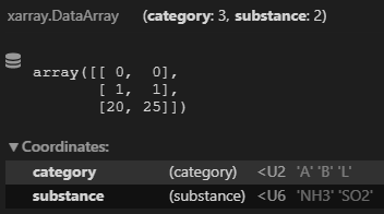
The first option requires to create a data array containing the profile index to use for any combination of the following coordinates :
category: a str matching the name of a category
substance: a str matching the name of a substance
cell : an integer matching the index of a cell
time : a datetime object matching the time of the emission (not implemented yet)
country : the 3 letter code of a country
type : [‘gridded’, ‘shapped’] depending if applies to gridded or shapped emissions
day_type : depending on the day of the week that the profile applies to
The coordinates don’t need to all be present in the file, one could simply put one of them, and emiproc assumes the vertical profiles are the same no matter the other coordinates. The profiles are then assinged to the inventory using the attributes: v_profiles_indexes and t_profiles_indexes.
The following image shows an example of how the indexes xarray.DataArray looks like:
Shapes Emissions
The second method applies to the shapes from the inv.gdfs . One column of each gdfs can be called __v_profile__ and __t_profile__ for the vertical and time profiles. Each shape of the gdfs can then be assigned to a desired profile. These columns contain the index of the profile assigned to that shape.
If these profiles columns are not set, emiproc assumes the profiles are the same as in the gridded emissions.
Behaviour during Operations
When calling an operator on the inventories emiproc handles operations on the profiles as well. As this is done in the background, we recommend you to keep track of what happpens to the profiles during operations.
If you see any suspicious behaviour, please report it as an issue on github .
Note
For developpers:
Operations on inventories can be tricky. The principle is to always weight correctly the different ratios. Sometimes arbitrary decisions have to be done. For example when adding two inventories, we need to decide if we use the vertical scales of on of the two, or if we want to go for a fancy merging.
Uncertainty on time profiles
Sometimes profiles are given uncertainty values. This is currently not handled in emiproc.
One would have to make sure the uncertainty propagate correctly while merging.
Examples
More examples can be found direclty in the inventories.
For example in tno.py the profiles are added to the inventory object using different emiproc functions.
Vertical profile based on roof heights
Warning
This example is not yet implemented, but we plann to show a test case using data for zurich.
Adding an elevation to each source
Instead of a vertical profile, one can also add an elevation to each source
as a point.
This can be done using the EmissionInfo class.
You can check an example for that the zurich inventory: categories_info.py