EDGAR Temporal profiles

This tutorial demonstrates how to use the auxiliary temporal profiles from edgar.

The function we will use is :py:func:emiproc.inventories.edgar.temporal.read_edgar_auxilary_profiles.

Loading EDGAR

Similarly to the EDGAR tutorial, we first load the inventory.

from pathlib import Path
from emiproc.inventories.edgar import download_edgar_files
from emiproc.inventories.edgar import EDGARv8

year = 2022

local_dir = Path("./edgar") / str(year)
local_dir.mkdir(exist_ok=True, parents=True)

# download_edgar_files(local_dir, year=year, substances=["CH4", "CO2", "CO2bio"])
inv = EDGARv8(
    local_dir / "EDGAR_*.nc",
    year=year,
    # Use short names, as this is how they are defined in the axilary table
    use_short_category_names=True,
)
inv

Inventory(EDGARv8)

Download the auxilliary data

Now you have to make a manual step to download the auxilliary data from EDGAR website.

You can find the auxilliary_tables.rar file at https://edgar.jrc.ec.europa.eu/dataset_temp_profile

Download it and extract its files in a local directory. You should have 4 .csv files.

Read the profiles

from emiproc.inventories.edgar.temporal import read_edgar_auxilary_profiles

path_to_auxiliary_filesdir = Path("/home/coli/Data/emiproc/aux_edgar/")
profiles, indices = read_edgar_auxilary_profiles(
    auxiliary_filesdir=path_to_auxiliary_filesdir,
    inventory=inv,
)

What is in the profiles ?

There are two components to emiproc profiles:

• the profiles themselves, which are objects of different temporal profile classes.

• the indices, a xarray dataset that tells for each sector/pollutant/gridcell/… which profile to use.

profiles

CompositeProfiles(76 profiles from ['HourOfWeekPerMonthProfile', 'WeeklyProfile'])

We have 2 types of profiles:

Weekly profiles that specify for each weekday how much of emissions are there.

HourOfWeekPerMonth: which sounds scary, but it means that for each hour of a week there is a profile value and also for each month this value is different.

indices

<xarray.DataArray (country: 234, category: 24)> Size: 45kB
array([[40, 63, 52, ...,  3, 24, 24],
       [10, 39, 34, ...,  4, 16, 16],
       [40, 63, 52, ...,  3, 24, 24],
       ...,
       [40, 63, 52, ...,  3, 24, 24],
       [40, 63, 52, ...,  3, 24, 24],
       [40, 63, 52, ...,  3, 24, 24]], shape=(234, 24))
Coordinates:
  * category  (category) object 192B 'ENE' 'CHE' ... 'TNR_Aviation_CRS'
  * country   (country) object 2kB 'ABW' 'AFG' 'AGO' 'AIA' ... 'PSE' 'ATA' 'ATF'

xarray.DataArray

• country: 234
• category: 24

• 40 63 52 63 63 6 6 41 6 5 63 63 6 ... 6 36 24 24 24 45 5 5 63 3 24 24

  array([[40, 63, 52, ...,  3, 24, 24],
         [10, 39, 34, ...,  4, 16, 16],
         [40, 63, 52, ...,  3, 24, 24],
         ...,
         [40, 63, 52, ...,  3, 24, 24],
         [40, 63, 52, ...,  3, 24, 24],
         [40, 63, 52, ...,  3, 24, 24]], shape=(234, 24))

• Coordinates: (2)
  • category
    (category)
    object
    'ENE' 'CHE' ... 'TNR_Aviation_CRS'

    array(['ENE', 'CHE', 'TRO', 'NMM', 'IND', 'AWB', 'ENF', 'NEU', 'AGS', 'WWT',
           'IRO', 'NFE', 'MNM', 'RCO', 'TNR_Ship', 'TNR_Aviation_CDS', 'TNR_Other',
           'PRO_FFF', 'SWD_LDF', 'SWD_INC', 'PRU_SOL', 'REF_TRF',
           'TNR_Aviation_LTO', 'TNR_Aviation_CRS'], dtype=object)

  • country
    (country)
    object
    'ABW' 'AFG' 'AGO' ... 'ATA' 'ATF'

    array(['ABW', 'AFG', 'AGO', ..., 'PSE', 'ATA', 'ATF'],
          shape=(234,), dtype=object)

In the indices, we have a 2 dimensional array with country and category as dimensions.

This means that each country and emission category can have a different temporal profile.

Set the profiles to the inventory

Now that we have loaded the profiles, we can set them to the inventory.

inv.set_profiles(
    profiles=profiles,
    indexes=indices,
)
inv.t_profiles_indexes

<xarray.DataArray (country: 234, category: 24)> Size: 45kB
array([[40, 63, 52, ...,  3, 24, 24],
       [10, 39, 34, ...,  4, 16, 16],
       [40, 63, 52, ...,  3, 24, 24],
       ...,
       [40, 63, 52, ...,  3, 24, 24],
       [40, 63, 52, ...,  3, 24, 24],
       [40, 63, 52, ...,  3, 24, 24]], shape=(234, 24))
Coordinates:
  * category  (category) object 192B 'ENE' 'CHE' ... 'TNR_Aviation_CRS'
  * country   (country) object 2kB 'ABW' 'AFG' 'AGO' 'AIA' ... 'PSE' 'ATA' 'ATF'

xarray.DataArray

• country: 234
• category: 24

• 40 63 52 63 63 6 6 41 6 5 63 63 6 ... 6 36 24 24 24 45 5 5 63 3 24 24

  array([[40, 63, 52, ...,  3, 24, 24],
         [10, 39, 34, ...,  4, 16, 16],
         [40, 63, 52, ...,  3, 24, 24],
         ...,
         [40, 63, 52, ...,  3, 24, 24],
         [40, 63, 52, ...,  3, 24, 24],
         [40, 63, 52, ...,  3, 24, 24]], shape=(234, 24))

• Coordinates: (2)
  • category
    (category)
    object
    'ENE' 'CHE' ... 'TNR_Aviation_CRS'

    array(['ENE', 'CHE', 'TRO', 'NMM', 'IND', 'AWB', 'ENF', 'NEU', 'AGS', 'WWT',
           'IRO', 'NFE', 'MNM', 'RCO', 'TNR_Ship', 'TNR_Aviation_CDS', 'TNR_Other',
           'PRO_FFF', 'SWD_LDF', 'SWD_INC', 'PRU_SOL', 'REF_TRF',
           'TNR_Aviation_LTO', 'TNR_Aviation_CRS'], dtype=object)

  • country
    (country)
    object
    'ABW' 'AFG' 'AGO' ... 'ATA' 'ATF'

    array(['ABW', 'AFG', 'AGO', ..., 'PSE', 'ATA', 'ATF'],
          shape=(234,), dtype=object)

Grouping Categories

When groupping categories, the profiles are automatically groupped.

This is done by a weighted average, so that categories with more emissions have more weight in the average during groupping.

from emiproc.inventories.utils import group_categories


grouped = group_categories(
    inv,
    categories_group={
        "agriculture": [
            # Agriculture
            "ENF",  # Enteric fermentation
            "MNM",  # Manure management
            "AWB",  # Agricultural waste burning
            "AGS",  # Agricultural soils
            "N2O",  # Indirect N2O emissions from agriculture
            "IDE",  # Indirect emissions from NOx and NH3
        ],
        "industry": [
            "ENE",  # Power Industry
            "REF_TRF",  # Refineries
            "IND",  # Combustion for manufacturing
            "RCO",  # Energy for buildings
            "PRO_FFF",  # Fuel exploitation
            "NMM",  # Non-metallic minerals production
            "CHE",  # Chemical processes
            "IRO",  # Iron and steel production
            "NFE",  # Non-ferrous metals production
            "NEU",  # Non-energy use of fuels
            "PRU_SOL",  # Solvents and products use
        ],
        "waste": [
            "SWD_LDF",  # Solid waste landfills
            "SWD_INC",  # Solid waste incineration
            "WWT",  # Waste water handling
        ],
        "transportation": [
            "TNR_Aviation_CDS",
            "TNR_Aviation_CRS",
            "TNR_Aviation_LTO",
            "TNR_Aviation_SPS",
            "TNR_Other",
            "TNR_Ship",
            "TRO",  # Road transport
        ],
    },
    ignore_missing=True,
)
grouped.t_profiles_indexes.coords

Coordinates:
  * category  (category) object 32B 'agriculture' ... 'transportation'
  * country   (country) object 2kB 'ABW' 'AFG' 'AGO' 'AIA' ... 'PSE' 'ATA' 'ATF'

Now the profiles are given for the grouped categories.

Remapping

The profiles are defined per countries, but the inventory is given on a grid. If we want to export the inventory with the profiles, we can remap the profiles onto the grid of the inventory.

First we will remap edgar to a coarser grid to speed up the process.

from emiproc.grids import RegularGrid
from emiproc.regrid import remap_inventory


grid = RegularGrid(xmin=-12, xmax=48, ymin=32, ymax=72, nx=60, ny=40)
remapped = remap_inventory(grouped, grid)

/home/coli/Documents/Projects/emiproc/emiproc/regrid.py:251: UserWarning: Geometry is in a geographic CRS. Results from 'area' are likely incorrect. Use 'GeoSeries.to_crs()' to re-project geometries to a projected CRS before this operation.

  gdf_weights.geometry_inter.area / gdf_weights.geometry.area

from emiproc.inventories.utils import country_to_cells


celled = country_to_cells(remapped)
celled.t_profiles_indexes.coords

89.6%

Coordinates:
  * category  (category) object 32B 'agriculture' ... 'transportation'
  * cell      (cell) int64 19kB 0 1 2 3 4 5 6 ... 2394 2395 2396 2397 2398 2399

Now we have a profile for each cell of the inventory

Generate time series

from emiproc.exports.hourly import get_temporally_scaled_array
import pandas as pd

da = get_temporally_scaled_array(
    inv=celled,
    time_range=pd.date_range("2022-01-01", "2022-01-14", freq="h"),
    sum_over_cells=False,
)
da.coords

Coordinates:
  * substance  (substance) <U6 72B 'CH4' 'CO2' 'CO2bio'
  * category   (category) object 32B 'agriculture' 'waste' ... 'transportation'
  * cell       (cell) int64 19kB 0 1 2 3 4 5 6 ... 2394 2395 2396 2397 2398 2399
  * time       (time) datetime64[ns] 3kB 2022-01-01 ... 2022-01-14

# Output is kg/year/cell, so we need to convert the units to kg/h/cell
from emiproc.profiles.temporal.constants import N_HOUR_YEAR

da /=  N_HOUR_YEAR

da.sel(substance="CO2", category="transportation").sum(dim="cell").plot(x='time')

[<matplotlib.lines.Line2D at 0x72ba658b6db0>]

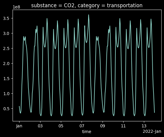
There we can see our temporal profile on the domain.

Conclusion

In this tutorial, we learned how to read EDGAR temporal profiles and combine them to the inventory.

If you have any questions, please refer to our support page.